tessellationrobot.github.io
Damping
## The goal of this test is to check the possible due the material that we used for creating the system.

## To evaluate this, we have attached 2 metal bars at the bottom of
## the system and we had hinged the system from the top. The metal bars
## were of 45 grams of weight each. The dimension of the bar is
## 80.6mm x 22.5mm x 3mm. The distance of center of mass from the axis of rotation is 70.7mm.

## We had attached a reference above the testing part link system for tracking in the video to evaluate the values.
Experimental Setup

We have exported the data from the video and then have performed the test below.
!pip install pynamics
import pandas as pd
import numpy
import matplotlib.pyplot as plt
import scipy.interpolate as si
import pynamics
from pynamics.system import System
from pynamics.frame import Frame

system = System()
pynamics.set_system(__name__,system)

A = Frame('A',system);
Collecting pynamics
Downloading pynamics-0.2.0-py2.py3-none-any.whl (87 kB)
[K |████████████████████████████████| 87 kB 2.7 MB/s
[?25hRequirement already satisfied: scipy in /usr/local/lib/python3.7/dist-packages (from pynamics) (1.4.1)
Requirement already satisfied: matplotlib in /usr/local/lib/python3.7/dist-packages (from pynamics) (3.2.2)
Requirement already satisfied: numpy in /usr/local/lib/python3.7/dist-packages (from pynamics) (1.21.5)
Requirement already satisfied: sympy in /usr/local/lib/python3.7/dist-packages (from pynamics) (1.7.1)
Requirement already satisfied: cycler>=0.10 in /usr/local/lib/python3.7/dist-packages (from matplotlib->pynamics) (0.11.0)
Requirement already satisfied: python-dateutil>=2.1 in /usr/local/lib/python3.7/dist-packages (from matplotlib->pynamics) (2.8.2)
Requirement already satisfied: pyparsing!=2.0.4,!=2.1.2,!=2.1.6,>=2.0.1 in /usr/local/lib/python3.7/dist-packages (from matplotlib->pynamics) (3.0.7)
Requirement already satisfied: kiwisolver>=1.0.1 in /usr/local/lib/python3.7/dist-packages (from matplotlib->pynamics) (1.4.0)
Requirement already satisfied: typing-extensions in /usr/local/lib/python3.7/dist-packages (from kiwisolver>=1.0.1->matplotlib->pynamics) (3.10.0.2)
Requirement already satisfied: six>=1.5 in /usr/local/lib/python3.7/dist-packages (from python-dateutil>=2.1->matplotlib->pynamics) (1.15.0)
Requirement already satisfied: mpmath>=0.19 in /usr/local/lib/python3.7/dist-packages (from sympy->pynamics) (1.2.1)
Installing collected packages: pynamics
Successfully installed pynamics-0.2.0
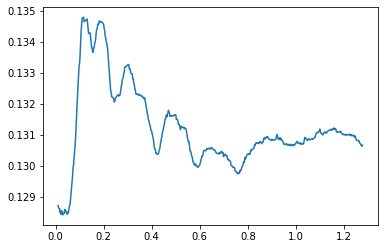
#load data from file and generate initial plots
df=pd.read_csv(r'Final2.txt', sep=',')
#print(df)
#x = df.x.astype('float64').to_numpy()
x = df.x.to_numpy()
y = df.y.to_numpy()
t1 = df.t.to_numpy()
x1 = df.a.to_numpy()
y1 = df.b.to_numpy()
x2 = df.c.to_numpy()
y2 = df.d.to_numpy()
tfactor = 30/480 #30fps video recored at 480 fps
t1=t1*tfactor
plt.figure()
plt.plot(t1,x)
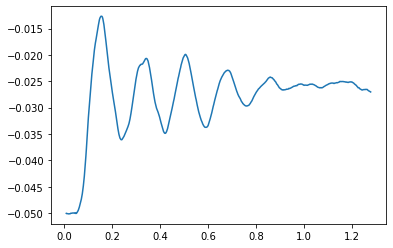
plt.figure()
plt.plot(t1,y)
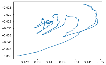
plt.figure()
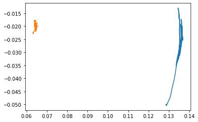
plt.plot(x,y)
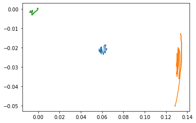
plt.figure()
plt.plot(x1,y1,x,y,x2,y2)
[<matplotlib.lines.Line2D at 0x7f3e3ac9f350>,
 <matplotlib.lines.Line2D at 0x7f3e3ac9f590>,
 <matplotlib.lines.Line2D at 0x7f3e3ac9f750>]
x -= x2
y -= y2
x1 -= x2
y1 -= y2
plt.plot(x,y,x1,y1)
[<matplotlib.lines.Line2D at 0x7f3e3a6b90d0>,
 <matplotlib.lines.Line2D at 0x7f3e3a6b9310>]
#convert data to angle data
#define vectors from center of servo to tip

vectx = x-x1
vecty = y-y1
vect = vectx*A.x+vecty*A.y
refvect = vect[0]
#use dot product + arccos to extract angle
angle = [1.0*(refvect.dot(item)/(refvect.length()*item.length()))  for item in vect]
#change data type for arccos function then convert to degrees
angles = (180/numpy.pi)*numpy.arccos(numpy.array(angle).astype(numpy.float64))
anglesrad = numpy.arccos(numpy.array(angle).astype(numpy.float64))
plt.plot(t1,angles)
plt.grid(True)
plt.xlabel("time in seconds")
plt.ylabel("angle in degrees")
#final angle 164.3 degrees from starting position
Text(0, 0.5, 'angle in degrees')
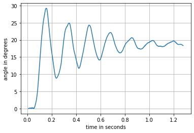
As seen in the graph above the servo dose not quite reach 180 degress this will be acounted for by comanding the model to go to the servo’s final angle of 164.3 degrees or 2.868 radians.
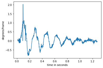
# angular velocity to find max angular velocity
speed = []
anglesL = angles.tolist()
for i in range(len(anglesL)):
speed.append(angles[i] - angles[i-1])
plt.figure()
plt.plot(t1,speed)
plt.xlabel("time in seconds")
plt.ylabel("degrees/frame")
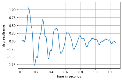
#clean derivative data with 7 point moving average
speedAVG = []
for i in range(3,len(speed)-3):
speedAVG.append((speed[i] + speed[i-1]+speed[i-2]+ speed[i-3] +speed[i+1]+speed[i+2]+ speed[i+3])/7)
plt.figure()
plt.plot(t1[3:727],speedAVG)
plt.grid(True)
plt.xlabel("time in seconds")
plt.ylabel("degrees/frame")
Text(0, 0.5, 'degrees/frame')
#Dynamics
from pynamics.frame import Frame
from pynamics.variable_types import Differentiable,Constant
from pynamics.system import System
from pynamics.body import Body
from pynamics.dyadic import Dyadic
from pynamics.output import Output,PointsOutput
from pynamics.particle import Particle
from pynamics.constraint import AccelerationConstraint
import pynamics.integration
from math import pi
lC = Constant(0.06604,'lC',system)
lD = Constant(0.0889,'lD',system)

mC = Constant(0.0028799999999999997,'mC',system)
mD = Constant(0.002216,'mD',system)

g = Constant(9.81,'g',system)
b = Constant(1e-4,'b',system)
k = Constant(1e-2,'k',system)

preload1 = Constant(-80*pi/180,'preload1',system)
preload2 = Constant(0*pi/180,'preload2',system)

Ixx_C = Constant(1e-2,'Ixx_C',system)
Iyy_C = Constant(1e-2,'Iyy_C',system)
Izz_C = Constant(5.420568769248424e-07,'Izz_C',system)
Ixx_D = Constant(1e-2,'Ixx_D',system)
Iyy_D = Constant(1e-2,'Iyy_D',system)
Izz_D = Constant(9.437043491466668e-08,'Izz_D',system)
#3 state variables:
qC,qC_d,qC_dd = Differentiable('qC',system)
qD,qD_d,qD_dd = Differentiable('qD',system)
initialvalues = {}
initialvalues[qC]=(180-51)*pi/180 ## Calculated using a protractor
initialvalues[qC_d]=0*pi/180
initialvalues[qD]=(90+24)*pi/180
initialvalues[qD_d]=0*pi/180
statevariables = system.get_state_variables()
ini = [initialvalues[item] for item in statevariables]
N = Frame('N',system)
C = Frame('C',system)
D = Frame('D',system)
system.set_newtonian(N)
#legs attached to the body
C.rotate_fixed_axis(N,[0,0,1],qC,system)

#legs attacheced to legs
D.rotate_fixed_axis(C,[0,0,1],qD,system)
pNO=0*N.x

pNC = pNO+lC*C.x
pCD = pNC+lD*D.x
pCcm = lC/2*C.x
pDcm = pCD - lD/2*D.x
#Angular velocity
wNC = N.get_w_to(C)
wCD = C.get_w_to(D)
IC = Dyadic.build(C,Ixx_C,Iyy_C,Izz_C)
ID = Dyadic.build(D,Ixx_D,Iyy_D,Izz_D)

BodyC = Body('BodyC',C,pCcm,mC,IC,system)
BodyD = Body('BodyD',D,pDcm,mD,ID,system)
system.addforce(-b*wCD,wCD)
<pynamics.force.Force at 0x7f3e3a2f9ad0>
system.add_spring_force1(k,(qD-preload2)*C.z,wCD)
(<pynamics.force.Force at 0x7f3e3a2eab90>,
 <pynamics.spring.Spring at 0x7f3e3a3e5790>)
system.add_constraint(AccelerationConstraint([-qC_dd]))
system.addforcegravity(-g*N.y)
f,ma = system.getdynamics()
2022-04-13 02:12:07,494 - pynamics.system - INFO - getting dynamic equations
func1,lambda1 = system.state_space_post_invert(f,ma,return_lambda = True)
2022-04-13 02:12:07,956 - pynamics.system - INFO - solving a = f/m and creating function
2022-04-13 02:12:08,085 - pynamics.system - INFO - substituting constrained in Ma-f.
2022-04-13 02:12:08,172 - pynamics.system - INFO - done solving a = f/m and creating function
2022-04-13 02:12:08,185 - pynamics.system - INFO - calculating function for lambdas
tol = 1e-5
tinitial = 0
tfinal = 1.2
fps = 480
tstep = 1/fps
t = numpy.r_[tinitial:tfinal:tstep]
states=pynamics.integration.integrate(func1,ini,t,rtol=tol,atol=tol, args=({'constants':system.constant_values},))
2022-04-13 02:14:44,786 - pynamics.integration - INFO - beginning integration
2022-04-13 02:14:45,058 - pynamics.integration - INFO - finished integration
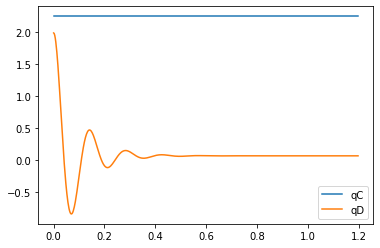
plt.figure()
artists = plt.plot(t,states[:,:2])
plt.legend(artists,['qC','qD'])
<matplotlib.legend.Legend at 0x7f3e351cd690>
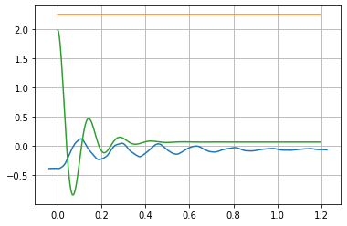
plt.plot(t1-.05,anglesrad-.39,t,states[:,:2])
plt.grid()
## What could you have done better in your experiment design and setup?

## The current material wich we have opted for, is an optimum material.
## So I do not feel there is any need to change the experiment design or the setup.
## While conducting the experiment, we have tried using the resources which were easily
## available nearby. But it we would have got a proper board,
## where we could pin the object properly, we would be able to
## visualize the experiment in a more better way.
## Discuss your rationale for the model you selected.
## Describe any assumptions or simplificaitons this model makes.
## Include external references used in selecting or understanding your model.
## Justify the method you selected (least squares, nonlinear least squares,
## scipy.optimize.minimize(), Evolutionary algorithm, etc. )
## for fitting experimental data to the model, as well as the specific algorithm used.

## I tried using the least square method but wasn't successful in obtaining the solution
## because of time constraints.
## How well does your data fit the model you selected? Provide a numerical
## value as well as a qualitative analysis, using your figure to explain.

## I have imagined that the model would mostly meet the requrement well looking at
## the final graph above.
## What are the limits of your model, within which you are confident of a good fit?
## Do you expect your system to operate outside of those limits?

## Our results have matched a lot with the numerical ones so I do not
## think there couldn't be a more better fit than this.
## Seeing the final graph, I assume that the system wouldn't operate outside the limit.